Simulating Classical Diversity Combining with Quantum Circuits

---

I am currently pursuing the Post-Graduate Diploma in Advanced Communication Engineering with Quantum and AI Integration at IIT Delhi (CEPQIP), and this post documents the first lab assignment in that programme. The goal was to implement three classical diversity-combining techniques — Selection Combining (SC), Equal Gain Combining (EGC), and Maximal Ratio Combining (MRC) — using Qiskit as the simulation runtime. If that sounds like an unusual pairing, it is. Qiskit is a quantum computing framework, not a wireless channel simulator. Making it behave like one required an explicit mapping between quantum measurement mechanics and classical communication concepts, and working through that mapping was the most valuable part of the exercise.

Why Use Quantum Circuits to Model Classical Channels?

The short answer is that a quantum circuit, at the level of abstraction used here, is a controlled probabilistic machine. You prepare a qubit in a known state, apply a transformation that introduces some rotation away from that state, measure the outcome, and record the probability of getting the original state back. That pipeline maps almost directly onto a classical communication link.

In this simulation, measuring the qubit in state

0⟩ represents a correctly received symbol. A deviation toward

1⟩ represents an error. The noise on the channel is modeled using a parameterized U gate — the most general single-qubit rotation, defined as:

U(θ, φ, λ) — a rotation on the Bloch sphere controlled by three angles

A larger rotation angle θ means more noise, which means a lower probability of measuring

0⟩, which means higher error rate. That is exactly the relationship you would expect from a degraded communication channel. The mapping is not physics — it is a deliberate analogy — but it is a productive one for building intuition about how combining strategies interact with channel quality variation.

Where the analogy works cleanly is in the diversity combining logic itself. Each branch is an independent circuit run with its own noise realization. SC picks the best branch. EGC averages equally across branches. MRC weights branches by quality. All three operations are mathematically identical to their classical counterparts; only the underlying “channel” is a qubit measurement rather than an RF signal.

Modeling Noise: From Fixed Angles to Rayleigh Fading

The assignment began with a simpler setup: four fixed-angle noisy channels with increasing rotation angles (θ = π/12, π/8, π/6, π/4), corresponding to noise levels of roughly 15°, 22.5°, 30°, and 45°. Running each circuit through the Aer simulator with 1024 shots gave measured probabilities of receiving

0⟩ of approximately 0.378, 0.324, 0.241, and 0.131 respectively — a clean monotonic decrease with noise strength, which validated the mapping.

The more interesting section was Rayleigh fading. In classical wireless systems, Rayleigh fading models channel gain as a random variable drawn from a Rayleigh distribution. I implemented this by sampling a fading gain at each SNR level and mapping it to a rotation angle using the relationship:

rayleigh_gain = np.random.rayleigh(scale=np.sqrt(snr_linear) * 0.2) theta = np.pi / 2 * np.exp(-rayleigh_gain)

The intuition behind this mapping: at high SNR, the expected gain is large, which drives theta toward zero, which means less rotation away from

0⟩, which means lower BER. At low SNR, theta approaches π/2 and error rates rise toward 0.5 — the maximum confusion level for a single-qubit measurement. This matches the expected SNR-BER relationship in classical Rayleigh fading channels, making the simulation behaviorally consistent with textbook wireless theory even though the underlying mechanism is a quantum circuit.

Diversity Combining Results: What the Simulation Showed

The main experiment swept SNR from 0 dB to 30 dB in 3 dB steps, averaged over 20 independent trials per point, and recorded BER for L = 2, 3, and 4 branches across all three combining techniques.

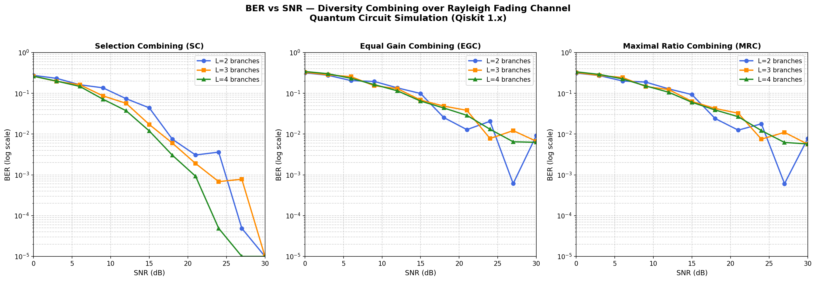Figure 1: BER versus SNR for SC, EGC, and MRC across L = 2, 3, and 4 branches. Y-axis is log scale. Each subplot isolates one combining technique to show the branch-count effect clearly.

The first thing the plots confirm is the expected monotonic BER decline with SNR across all three techniques and all branch counts. That is the sanity check — without it, the simulation mapping would be suspect.

The more instructive result is the gap between SC and the other two techniques. At L = 4 branches, SC drops to effectively zero BER by 24 dB SNR, while EGC and MRC remain in the 0.012–0.014 range at the same point. This is a large gap, and it is not because SC is a fundamentally superior algorithm. It is because of how SC is defined in this simulation: SC selects the branch with the minimum measured BER, which is an optimistic best-case selector. In a single-circuit-run experiment where each branch BER is estimated from 1024 shots, the minimum is inherently a downward-biased estimate. SC wins in this formulation partly because the formulation gives it the statistical high ground.

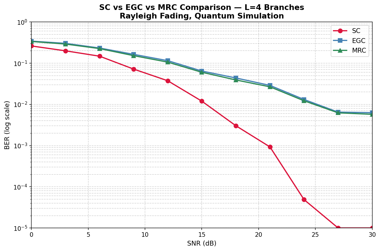
Figure 2: SC versus EGC versus MRC for the 4-branch case. SC separates sharply at high SNR. EGC and MRC track within a few percent of each other throughout the sweep.

The second notable result is how closely MRC tracks EGC. In theory, MRC should outperform EGC because it uses channel state information to weight stronger branches more heavily. In this simulation, that advantage is present but small — typically a few percent below EGC in BER at matching SNR points. The reason is that per-branch BER estimates derived from a single circuit run are noisy. When branch quality estimates are similar (which happens often after averaging over 20 runs), MRC’s weighting adds little information over EGC’s uniform average. The MRC advantage would likely be more visible with more shots per circuit or with branches that have more divergent fading realizations.

The simulation does not show MRC is weak — it shows that MRC’s advantage over EGC depends on the reliability of per-branch quality estimates. In this experiment, those estimates are noisy enough to compress the gap.

QBER: A Glimpse Into the Next Dimension

The assignment also included a second phase of experiments measuring Quantum Bit Error Rate (QBER) — the probability of measuring an incorrect state under two noise models (depolarizing and phase-flip) across five gate types (U, H, X, S, T) and qubit counts from 1 to 5. The results there reveal something that classical communication engineers would find counterintuitive: phase-flip noise is consistently approximately twice as damaging as depolarizing noise across comparable conditions, and the H gate produces near-random QBER (~0.5) regardless of noise strength.

Those findings warrant their own detailed treatment. I will cover the full QBER analysis — including the gate-by-gate breakdown and what it implies for noise model selection in quantum channel simulations — in the next post in this series.

What the Analogy Gets Right (and Wrong)

Being honest about the limits of this simulation matters, particularly if you are coming from a classical wireless background and wondering whether this approach generalises.

What it gets right: the qualitative behavior of all three combining techniques is preserved. SC outperforms the averaging strategies at high SNR. More diversity branches reduce BER. The SNR-BER trend matches classical Rayleigh fading theory. The circuit abstraction is coherent and internally consistent.

What it does not get right: MRC in this implementation is a weighted average of measured BER values, not a coherent combiner that operates on received signal amplitudes. In a real MRC receiver, combining happens in the signal domain before detection — it is fundamentally a pre-detection operation. Here, combining happens on post-measurement probabilities. This is an educational approximation, not a hardware-accurate model. Similarly, shot noise from finite circuit runs affects every branch BER estimate, which means the simulation has a noise floor that a real system would not have in the same form.

The right way to think about this simulation is as a probabilistic laboratory for building intuition about diversity combining behavior. It is not a substitute for link-level simulation in tools like MATLAB or ns-3, and it does not predict real-system performance. What it does do is make the logic of combining strategies tangible in a way that is easy to instrument, modify, and extend — which, for learning purposes, is exactly what you want. The full Qiskit Aer noise modeling documentation covers the noise model API in detail, including how depolarizing and Pauli errors are constructed — worth reading if you want to extend this simulation beyond the basics —

Key Takeaways

• A quantum circuit can serve as a controlled probabilistic channel simulator: U-gate rotation angle maps to noise strength, and measurement probability maps to signal fidelity. The analogy is pedagogically valid but not hardware-accurate.
• SC’s dominance in this simulation is partly a definitional artifact — selecting the minimum branch BER is an optimistic estimator. Interpret cross-technique comparisons with that in mind.
• MRC’s advantage over EGC compresses when per-branch quality estimates are noisy. More shots per circuit or more divergent fading realizations would widen the gap.
• Phase-flip noise is more damaging than depolarizing noise in the X-basis measurement setup used here — a result that does not have a classical intuition and deserves its own analysis.
• Qiskit’s Aer simulator is a practical tool for this kind of exploratory work, but the deprecated execute() API needs replacing with AerSimulator().run() in Qiskit 1.x.

---

Harshit is an Associate Principal Engineer with a decade of experience in enterprise-scale distributed systems, currently pursuing the Post-Graduate Diploma in Advanced Communication Engineering with Quantum and AI Integration at IIT Delhi (CEPQIP). This post documents lab work from that programme.

---

Ideation and creation by human, written and formatted by AI